384 residues · 1,536 backbone atoms · 500 frames
HelixSheetLoopStarting conformation
An interactive, precomputed all-backbone example from the current DynaMode work. The paper and benchmarks below describe the original Cα model.
Why model motion?
A structure captures one conformation of a protein. Understanding its behaviour also means understanding the states it can visit and how it moves between them. Molecular dynamics simulations offer this view, but they are expensive; many generative approaches instead produce collections of conformations without an explicit time ordering.
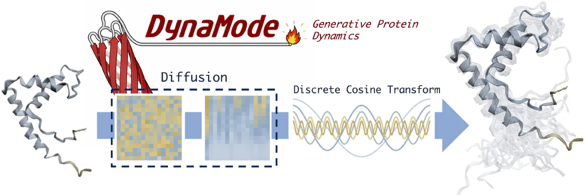
DynaMode asks whether we can learn a whole window of motion at once. Given a monomer structure and temperature, the published model generates a temporally ordered Cα trajectory by predicting its frequency representation. The aim is a fast way to explore dynamics while keeping slow collective changes and faster fluctuations within the same model.
From motion to frequencies
We express each residue’s movement relative to the input structure and apply a discrete cosine transform (DCT-II) along time. This turns its x, y and z displacement traces into frequency coefficients: low frequencies describe slower changes, while higher frequencies describe faster variation between sampled frames. The zero-frequency term captures mean displacement; power in the remaining frequencies relates directly to residue flexibility.
A diffusion model learns to denoise these spectral volumes, conditioned on the structure and temperature. Its spectral-convolution architecture mixes frequency bands and uses a dedicated low-frequency correction branch to improve the amplitudes most closely associated with flexibility. An inverse DCT then converts the prediction back into a window of structures. We retain the full spectrum: discarding the higher frequencies damaged structural geometry even when broad flexibility profiles survived.
What it learns from
The paper uses mdCATH, a dataset of 5,398 monomer domains simulated at five temperatures from 320 to 450 K. Training samples 256-frame windows at 1 ns spacing, with residue crops of 576. Evaluation includes 495 held-out mdCATH domains and 82 ATLAS targets at 300 K; ATLAS is outside both the training dataset and temperature range. These details refer to the paper’s Cα model, rather than the all-backbone example above. Methods, sections 3–4.
What the results show
On mdCATH, DynaMode has the highest pairwise-RMSD and global-RMSF correlations among the non-oracle methods in Table 1. The picture is mixed across other metrics: it does not lead the ensemble-distance measures. The tables below reproduce selected columns from the paper, retaining every method in each table.
Held-out mdCATH · 320–450 K
| Method | Pairwise RMSD r ↑ | Global RMSF r ↑ | RMWD ↓ | PCA W₂ ↓ |
|---|---|---|---|---|
| Oracle | 0.992 | 0.885 | 3.08 | 2.21 |
| MDGen | 0.710 | 0.670 | 3.36 | 2.62 |
| AlphaFlow-MD | 0.410 | 0.410 | 5.62 | 2.38 |
| Tempo | 0.770 | 0.670 | 4.21 | 2.33 |
| DynaMode | 0.854 | 0.844 | 4.12 | 2.78 |
Selected columns from Table 1, aggregated over 2,475 test trajectories. Competitor values come from their published evaluations, rather than a fresh rerun of every model. Full table and protocol.
ATLAS · 300 K
| Method | Pairwise RMSD r ↑ | Global RMSF r ↑ | RMWD ↓ | PCA W₂ ↓ |
|---|---|---|---|---|
| Oracle | 0.835 | 0.910 | 1.85 | 1.25 |
| MDGen | 0.480 | 0.500 | 2.69 | 1.89 |
| AlphaFlow-MD | 0.480 | 0.600 | 2.61 | 1.52 |
| Tempo | 0.910 | 0.890 | 1.49 | 0.60 |
| DynaMode | 0.665 | 0.734 | 2.65 | 1.72 |
Selected columns from Table 2. This is an out-of-distribution test for DynaMode; the compared models train on subsets of ATLAS. Performance falls relative to mdCATH, with Tempo ahead on these metrics. Full table and protocol.
Reading the tables: ↑ means higher is better; ↓ means lower is better. RMSF measures residue flexibility, while pairwise RMSD reflects conformational variation. RMWD and PCA W₂ measure differences between generated and reference ensembles. The oracle is a reference-MD comparison, not a learned model. Bold identifies the DynaMode row, not the best score in every column.
Speed, geometry, and what comes next
The paper reports roughly one second to generate a 256-frame window on a GH200 GPU. Structural validity remains a limitation: confident motion predictions can introduce steric clashes. Post-generation energy minimisation improves geometry but substantially reduces the speed advantage. The small direct timing-and-validity comparison and the full trajectory benchmark are separate experiments; the mdCATH table uses predictions without energy minimisation.
The next challenge is to combine the spectral representation’s useful description of motion with stronger spatial reasoning. The current all-backbone example at the top illustrates ongoing work beyond the original Cα paper; its presence here does not establish equivalent benchmark performance. Discussion and limitations.
Summary and selected table columns adapted from Phipps et al., “Spectral Diffusion for Protein Dynamics”, arXiv:2607.04134v1 (5 July 2026), CC BY 4.0. See the paper for the complete results and GitHub for the code.